Quick start tutorial
Tutorial Summary
This tutorial will get you started using the RAMjET pipeline to train a neural network to detect exoplanet transit events in TESS data. You will end up with a trained neural network that can be applied to TESS lightcurves to predict if a transit exists in the given lightcurves. This tutorial is only intended to get the code working for you for a specific use case. It will not teach you how the process works nor how to make it work for another use case.
Install
First, you need Python 3.7 with pip installed (most Python 3.6+ versions should work, but some required packages
may not be available on newer verisons yet). Ideally, this Python install is in its own Python virtual
environment or Conda environment to make sure this project doesn’t interfere with other projects and vice versa. The
rest of this tutorial assumes the command python will run your Python 3 install (on some systems this will
run Python 2 by default). The same is true for pip running the Python 3 related version of pip.
Next, clone down the RAMjET repository and change directory to that repository:
git clone https://github.com/golmschenk/ramjet.git
cd ramjet
Then, you’ll need to install all the required Python packages:
pip install -r requirements.txt
This installation assumes you already have your GPU properly setup and installed, and the GPU is compatible with TensorFlow (if you intend to use a GPU). Note that without a GPU, the training code will take significantly longer to run.
Download the data
Next up, we need to get the TESS data to use for training and evaluation. To do this, from the ramjet directory,
run:
python -m ramjet.photometric_database.setup.quick_start
This download will take a while and will download ~25GB of data.
Train the network
To train the network, run the following command:
python train.py
If you run out of memory, reducing the batch size in train.py may help.
Training metrics will be printed to the terminal as the network learns. To see the live training progress in plot form,
open a second terminal in the ramjet directory and run:
tensorboard --logdir=logs
This will start a local web server which displays the training progress in plot form. With this running, the plots
can be viewed by opening a web browser to http://localhost:6006.
When the training finishes, or if you end it early with something like control + c, the trained network will
be saved to the log directory.
Using the trained network to make predictions
To use the network to make predictions over all the lightcurves, run:
python infer.py
This script will load the latest trained model (from the logs directory), and use it make a prediction about
each of the lightcurves. A number from 0 to 1 is assigned to each lightcurve which states the network’s confidence that
the lightcurve contains a transit event. 0 meaning the network is confident that the lightcurve contains no transit and
1 meaning the network is confident the lightcurve contains a transit. These predictions will be saved to a file in the
same log directory where the trained model is kept. By default, only the top 5,000 results are kept. The path to this
file from the root ramjet directory will be
logs/baseline YYYY-MM-DD-hh-mm-ss/infer results YYYY-MM-DD-hh-mm-ss.csv, where the first datetime is when
the network training was started, and the second datetime is when the inference run was started. The results will be
sorted with the most likely transit candidates at the stop of the list.
Viewing the predictions
To directly view one of the lightcurves, ramjet provides an quick viewing interface with something
like:
from ramjet.data_interface.tess_data_interface import TessDataInterface
tess_data_interface = TessDataInterface()
path_to_lightcurve = ''  # Replace this string with the path to the lightcurve.
tess_data_interface.show_lightcurve(path_to_lightcurve)
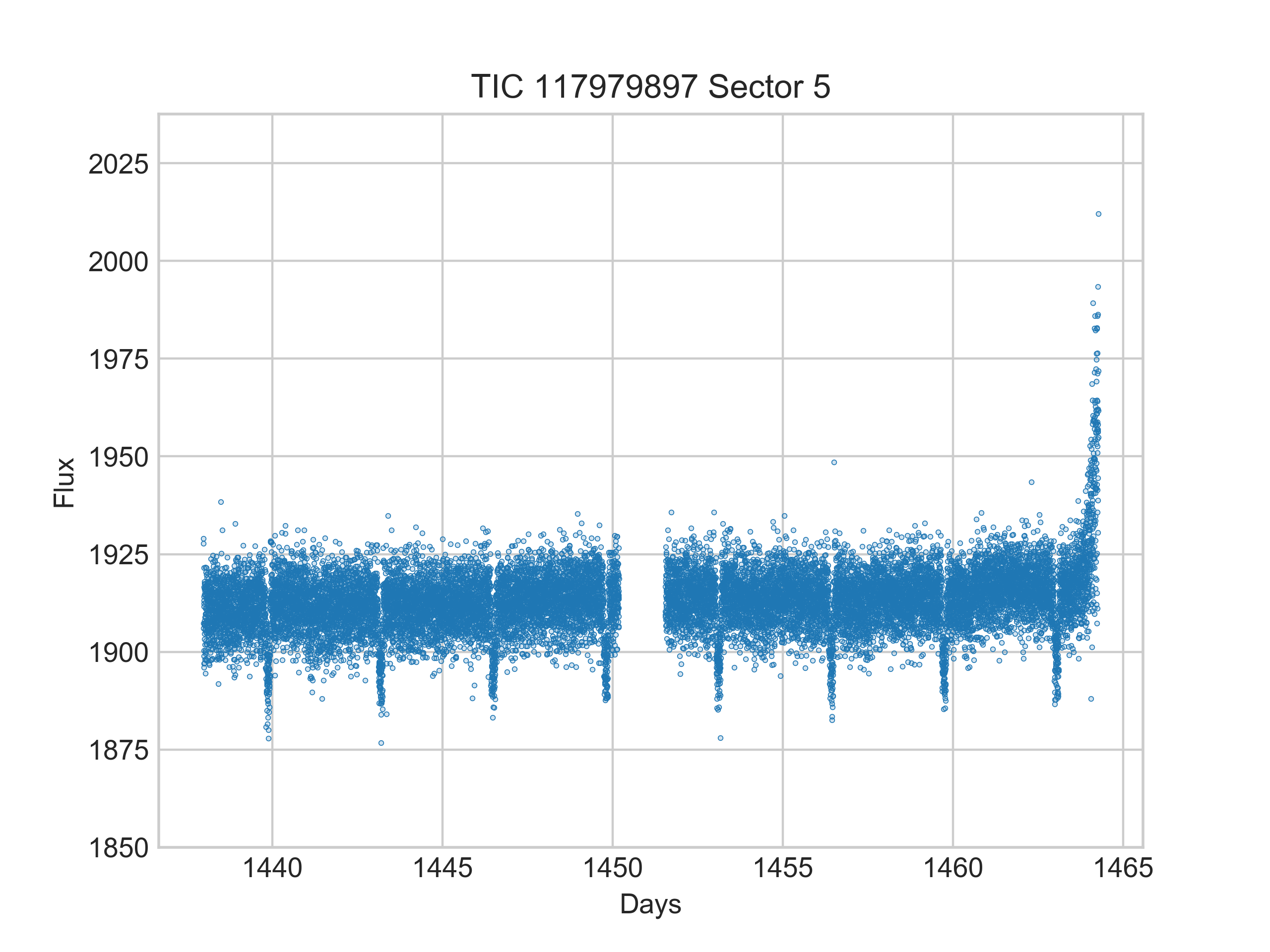
ramjet also provides a quick way to download and view any lightcurve available on MAST online using:
from ramjet.data_interface.tess_data_interface import TessDataInterface
tess_data_interface = TessDataInterface()
tess_data_interface.show_pdcsap_and_sap_comparison_from_mast(tic_id=117979897, sector=5)