Quick start tutorial¶

Tutorial Summary¶

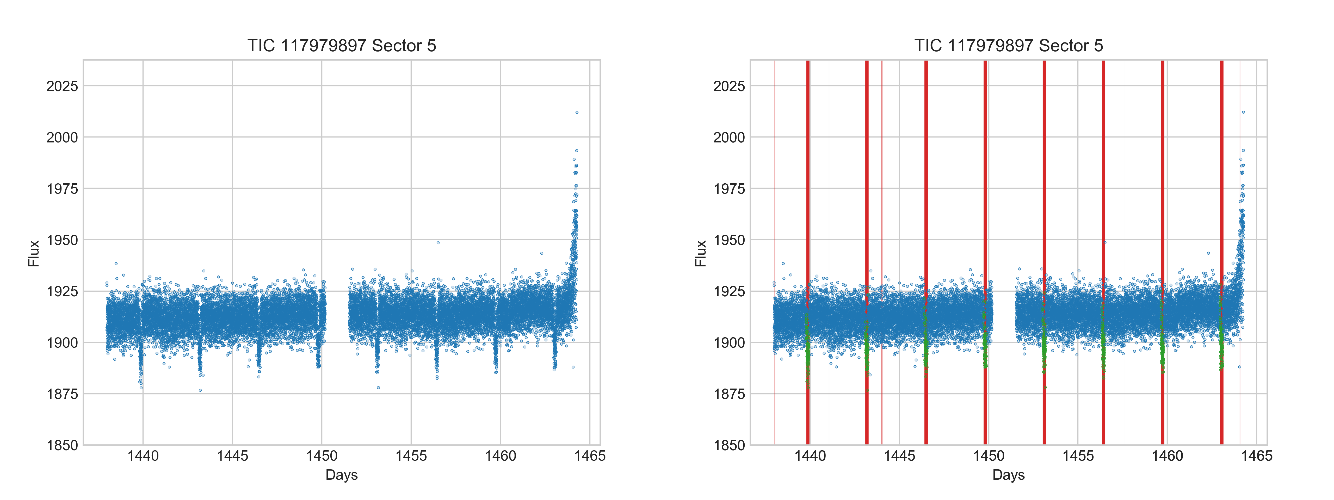
This tutorial will get you started using the RAMjET pipeline to train a neural network to detect exoplanet transit events in TESS data. You will end up with a trained neural network that can be applied to TESS lightcurves to predict where transits exist in the lightcurve (if they exist at all). For example, one of the below images show an original lightcurve from TESS, and the other shows the true transit locations (in green) as well as what the trained neural network predicted (in red). You will be able to produce results similar to this. This tutorial is only intended to get the code working for you for a specific use case. It will not teach you how the process works nor how to make it work for another use case.

_images/tess-lightcurve-with-transits-and-predictions.png

Install¶

First, you need Python 3.6+ with pip installed. Ideally, this Python install is in its own Python virtual environment or Conda environment to make sure this project doesn’t interfere with other projects and vice versa. The rest of this tutorial assumes the command python will run your Python 3 install (on some systems this will run Python 2 by default). The same is true for pip running the Python 3 related version of pip.

Next, clone down the RAMjET repository and change directory to that repository:

git clone https://github.com/golmschenk/ramjet.git
cd ramjet

Then, you’ll need to install all the required Python packages:

pip install -r requirements.txt

This installation assumes you already have your GPU properly setup and installed, and the GPU is compatible with TensorFlow (if you intend to use a GPU). Note that without a GPU, the training code will take significantly longer to run.

Download the data¶

Next up, we need to get the TESS data to use for training and evaluation. To do this, from the ramjet directory, run:

python -m ramjet.photometric_database.toi_lightcurve_database

This download will take a while and will download ~20GB of data.

Train the network¶

To train the network, run the following command:

python train.py

If you run out of memory, reducing the batch size in train.py may help.

Training metrics will be printed to the terminal as the network learns. To see the live training progress in plot form, open a second terminal in the ramjet directory and run:

tensorboard --logdir=logs

This will start a local web server which displays the training progress in plot form. With this running, the plots can be viewed by opening a web browser to http://localhost:6006.

When the training finishes, or if you end it early with something like control + c, the trained network will be saved to the log directory.

Using the trained network to make predictions¶

To make a prediction for a lightcurve like shown above, run:

python infer.py

This script will generate a plot of a lightcurve with the network’s predictions and save the image to a file in the current directory.

Although the network can make very predictions very quickly, this particular inference script is slowed by several factors. In particular, the network initialization (required only once for any number of predictions) and result image generation are relatively slow. Additionally, to keep the code simple, the data preprocessing is done synchronously with predictions, and the network processes a single lightcurve at a time. Asynchronous data preprocessing and predictions on batches of lightcurves leads to significantly faster inference speeds (but less understandable code, hence is excluded from this example script).